

PROJECT
Pub Crawler
Overview
For my computer science course, I had been tasked with making a ‘recommendation software’ in Python using a data structure & and algorithm. I left it and came back to it later, and decided to make a bit of a meal out of it. I wanted to attempt to stretch my skills a bit rather than checking off a project from the list, so here is my finished product: the pub crawler.
This solution is meant to simply take in your post code, a number, and it will recommend to you a series of pubs to visit in order. The files are available on my GitHub:
The components are:
– A data source of all pubs in the UK
– A means to return longitude and latitude from a postcode
– A way to filter down by pubs within a certain radius
– A graph data structure to store the pubs as vertices
– Calculation of the distance between all vertices
– A path-finding algorithm to traverse the graph to take an effective path to all pubs
Module Overview
Here is a list of all modules used in this project
Data Source
For this I used a dataset from Kaggle.
https://www.kaggle.com/datasets/rtatman/every-pub-in-england/data?select=open_pubs.csv
It fits my needs, and will provide a comprehensive data source to allow the location of the starting point to be dynamic.
Postcode. First I wanted to validate the that input was a proper UK postcode, which should be alpha numeric string between 5 and 7 digits / characters. Removing the space allows the regex match to work properly.
Next we initialise a map graph based on the postcode.
Then we use that graph and use Nominatim to return the longitude and latitude of the postcode.
If no location is returned, the program ends.
Next we check how many pubs the user intends to visit.
This section is very simply: is the input for num_of_pubs an int? If so, move on. If not, then it’s not a number.
Next we need to filter down the dataset. We don’t really care about pubs in the midlands if we’re in the south, so I think that reducing the pubs in the dataset before calculating distances would speed up the computer time dramatically, and it wouldn’t make practical sense to give the user hundreds of miles of pubs to choose from.
I created a filtered dataframe using the columns of the original. Then, for each row in the original dataframe, I take the longitude and latitude and take the difference by returning the absolute result of a subtraction of each. If the difference in longitude and latitude is less than or equal to 0.05, then it’s close enough to be considered. Changing the radius value to be higher will increase the range of pubs.
The Graph Data Structure
Firstly, we have to create the graph class. I initialised this from a different graph script I made.
The walking path function uses osmnx to find the nearest map nodes, and calculates the shortest distance using networkx.
The result of this code section, is that all pubs within a reasonable distance to your start postcode, and the start postcode, are all added to the graph data structure, and distances from each vertex to all other vertices is calculated as walking distance.
Pathfinding Algorithm
I originally wanted to use something like Djikstra’s or the A* pathfinding algorithms, but I quickly learned that it would be difficult without a target node to calculate in reference of. For this reason, I opted to take aspects of Djikstra’s algorithm and make my own pathfinding algorithm that prioritises relative distance between vertices, as well as their distance to the starting point. You don’t want to go out and end up far away from home, so keeping the distance to the start point seemed like a good idea.
Firstly, the scatter_map is initialised in the plotly.express module.
Then we return a list of the closest n pubs in order. This is from the graph.py script that gets imported at the start.
This algorithm returns the edge weights and neighbouring vertices of the home node, which will allow us to return the closest node, using the find_closest_node function.
It’s a very simply function to check and return the vertex with the smallest edge weight. If two or more vertices have the same smallest edge weight, the first is taken.
A path list is initialised with the closest path as the first item, and a visited list is initialised with the closest home vertex as the first item.
The closest vertex is set as current_vertex for the upcoming loop. The following loop is made possible by all vertices being connected to all other vertices. We loop through all neighbouring vertices that aren’t in the visited list and return the closest neighbour using an adjusted weight. That nearest vertex is added to the path, added to the visited list, and set as the current vertex.
The find_closest_adjusted_node function uses a relatively simple formula. For each neighbouring vertex (neighbour) of the current vertex, providing we haven’t already visited the node, and it’s not the home nose, and the edge weight is greater than 0 (showing a distance calculation error), then we find the distance of the neighbour from the home, and add to that the edge weight from the current vertex.
Then, if the adjusted distance is lower than the previous record, update the vertex and smallest number, and at the end of the loop, return the closest_vertex. This weights the neighbouring node by how far it is from the home vertex. This way, we don’t end up going in a straight line if a circular shape is reasonable.
Plotting Travel Lines
We need to find all longitude and latitude points for all nodes in order to generate the path lines, as that’s how the Scattermap works. We set the home latitude and longitude as the first items in the lists, then for each item in the closest_vertices list, we find their coordinates from the filtered_df and append those to the lists.
Finally, we add a trace over the existing map, and input the lat_values and lon_values. What this feature does, is plot a line from index 0 to 1, index 1 to 2 and so on. This makes a nice path. fig.show() your pub crawl is ready!
Testing
Test #1 – Eeny, meeny, miney, mo. Random finger on the map and away we go. Ashbourne Library, 4 pubs.
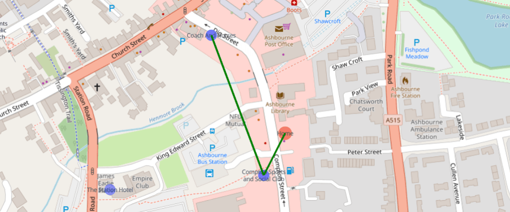
This looks like a failure – but wait! Analysis. The algorithm worked.
The first two location for some reason appear in the same place, but they are distinct places. The social club should be further down, but as they overlap on the map, it would make total sense to go next door to stop number 2.
The third and fourth stop are two pubs directly next to each other.


Test #2 – Picking another random point on the map – Galashiels interchange, 6 pubs
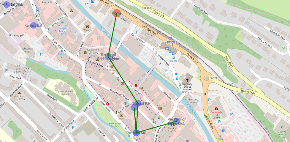
It might seem like the algorithm has gone a bit rogue and doubled back to an already visited node.


The Salmon Inn and The Auld Inn are relatively on top of each other on the map. There is a bit of strange behaviour how the nodes are positioned on the map versus where they actually are in real life. Investigating from the raw dataset, the coordinates aren’t 100% correct.
Test #3 – Finally, the Preston hotel in Yeovil, 9 pubs
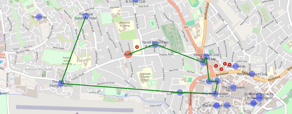
Now that, looks like a solid plan. You’ll notice that on the bottom right, there are a huge clump of pubs. In theory, the algorithm could be tweaked to predict clusters to improve path finding, but it did what it was meant to do – travel to close pubs one at a time, prioritising pubs that keep you close to where you started.
Optimisation
Now, I wrote this logic and code with the assumption that I was going to analyse the shortest path using something like the A* method, but as the project progressed, I realised that 1) That would be more for if I wanted to hit a target with the shortest path, which wouldn’t include keeping us close to home without modification, and 2) based on the algorithm I decided to implement, creating all edge weights before calculation is unnecessary.
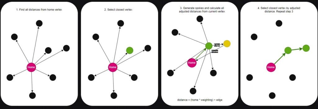
The spoke method I ended up using has the following steps:
1) Initially calculate all edge weights from the home position to all vertices
2) Check the adjusted distance from home for all nodes
3) Select the closest vertex by adjusted distance and add it to the visited list
4) Calculate edge weights to all uninvited vertices
5) Select the closest vertex by adjusted distance, add to the uninvited list and make it the active vertex
6) Loop back to step 3 unless the desired number of vertices have been discovered
In terms of runtime, calculating all edge weights would have a quadratic runtime of O(n^n), as all vertices have to be distance calculated in relation to all other vertices regardless of it they’re likely to be used or not. The optimisation after ‘completing’ the project that jumped out at me, and it sounds silly to me that this wasn’t obvious to me at the time, is that the runtime can be made much more efficient if edge weights were calculated on the chosen vertex. This would result in a runtime of O(log n), as we ignore vertices we’ve already travelled to each iteration. In the worst realistic case, if we have 10 pubs in the area and the user wants to travel to 10 pubs, the program flow will go something like: home checks 10 vertices, pub 1 checks 9 vertices, pub 2 checks 8 vertices and so on.
I ended up completely re-coding a decent portion of the script to make it work a little better, and removed a bunch of testing functions I wrote early on. Here is the V2 script.
Here is the updated function in the graph script to include weighting the adjusted distance. I set the weighting to 0.25 to allow home distance to influence the path, but ultimately, the actual distance between vertices is the main factor. This prevents the path from staying close to home but in the process, horribly sacrificing the overall distance.
Now that the script is optimised, I will attempt something that wasn’t possible before – a pub crawl in central London. There were too many pubs and it took forever, but we’ll see how long the optimised script takes for a 10 pub crawl, starting at the houses of parliament.
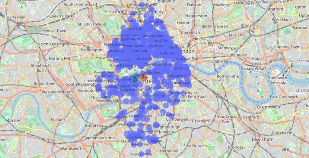
This script run took around 2.5 hours, and you can see why… It’s worth remembering that it populates the graph data structure and spokes out to other vertices every time it runs. If this were an actual web-based application, all of the connections would be pre-loaded into the backend so that the only compute needed would be to explore the graph.
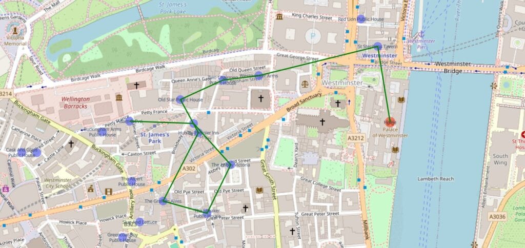
There we have it – a bit of a wait, but it finished. A 10 pub crawl starting from the houses of parliament. The original algorithm would have a quadratic runtime of O(n^2), because it calculated spokes for all items in relation to all other items. This modified version has a runtime of O(log n), as we reduce the steps needed for each vertex visited, making it more efficient.
Summary
I’d rate this project a huge success. I’m most happy that I designed my own path finding algorithm and it works fairly well. Some things if I were to do this again I’d improve/change might be to test a second or third potential path for the next spoke to check if the two-step process is shorter for each which would increase runtime by a fair amount but might produce better results. Additionally, for areas with a large concentration of pubs, I’d automatically reduce the search radius to make the script run faster.
I’m happy with this project, and it’s customisable to the point that you can simply adjust the weighting of the home distance in the adjustment calculation to fit your preference. Additionally, providing you can remap the columns, you can use your own CSV for anything you like – parks, restaurants, toilets – whatever you fancy.
One final thing I’d probably do on a second attempt would be to make it a GUI app rather than a script, but that’s for another time. Regardless, it’s an application that works and has a genuine use, and I even managed to optimise the algorithm to improve performance, so I’m happy.